Heatmaps
Functions for plotting heat- and clustermaps with seaborn. They are rather specific, and there might be better options in R or with PyComplexHeatmap.
# Block that has to be executed for all.
import Heatmaps
import seaborn as sns
out_dir = 'docs/gallery/'
penguin_df = sns.load_dataset('penguins')   # Example data from seaborn.
- Heatmaps.heatmap_cols(plot_df, cmap_cols, plot_out, row_label_col=None, column_labels=None, class_col=None, x_size=20, y_size=40, title='', annot_cols=None, width_ratios=None, wspace=0.4, rasterized=True, annot_s=10, ticksize=14, heat_ticksize=14, square=False, x_rotation=70, y_rotation=0, ax_fontweight='normal', row_label_first=False, formats=['pdf'])
Multiple heatmaps side-by-side but the same rows. Allows to show several metrics for the same rows with different colourmaps etc. E.g. for a list of top differential genes first a heatmap of baseline expression coloured by TPM, followed by a separate heatmap-block with the log2FC for the same genes.
- Parameters:
cmap_cols –
Dictionary with one entry for each block. The keys don’t matter as long as they are unique. E.g. {0: {‘cols’: [‘Mean_Control_FM’, ‘Mean_FM_Mock_Ctrl’, ‘Mean_Tcf15_FM’, ‘Mean_FM_Tcf15_OE’],
’centre’: 0, (optional) ‘cmap’: ‘mako’, ‘cbar_label’: ‘TPM’, ‘vmax’: 200, (optional) ‘vmin’: 0, (optional) }
row_label_col – Column where to fetch the row-strings from.
column_labels – Alternative to using the column names as indicated in cmap_cols.
class_col – Column that should be added as separate first heatmap-block, should be categorical.
annot_cols – Dictionary of {“column”: “column with annotation string”} to write the strings in the value into the cells of columns.
width_ratios – Ratios of the widths of each heatmap-block.
wspace – Additional horizontal space between blocks.
rasterized – Whether to draw thin white lines around cells.
square – Whether cells should be squares.
row_label_first – Only write the row names for the first entry and skip for the others.
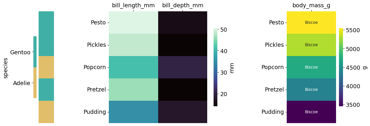
# Create a heatmap with several blocks that allow separate metrics to be shown side-by-side.
# For an example pick a few random rows and give them names so we can recognize them in the heatmaps.
sub_penguin_df = penguin_df.sample(5, random_state=12)
sub_penguin_df['Name'] = ['Pesto', 'Pickles', 'Popcorn', 'Pretzel', 'Pudding']
# Now we need to define which heatmap-blocks we want to show.
cmap_cols = {0: {'cols': ['bill_length_mm', 'bill_depth_mm'],
                 'cmap': 'mako',
                 'cbar_label': 'mm'},
             1: {'cols': ["body_mass_g"],
                 'cmap': 'viridis',  # Just for the sake of a different colour.
                 'cbar_label': 'g'}
             }
# We can additionally choose to add labels into cells, can be any other column.
annot_cols = {"body_mass_g": 'island'}
Heatmaps.heatmap_cols(sub_penguin_df, cmap_cols=cmap_cols, plot_out=out_dir+"SubPenguins", row_label_col='Name', class_col='species',
                 x_size=14, y_size=5, annot_cols=annot_cols, width_ratios=None, wspace=0.8,
                 annot_s=10, ticksize=14, heat_ticksize=14, square=False, x_rotation=0, formats=['png'])
- Heatmaps.clustermap(plot_df, columns, row_column, cbar_label, class_col='', class_row='', title='', plot_out='', vmin=None, vmax=None, annot_cols=None, cmap='viridis', x_size=12, y_size=10, y_dendro=False, x_dendro=True, column_labels=None, row_cluster=True, col_cluster=True, centre=None, tick_size=12, mask=None, metric='euclidean', z_score=None, class_col_colour=None, formats=['pdf'])
Create a heatmap that can be additionally clustered with seaborn. CARE: the class_col_order and class_row parameters are not properly tested.
- Parameters:
columns – List of the columns, should be present in the plot_df.
row_column – Column with which rows should be taken, set to ‘index’ to take the df.index.
class_col – Add a column into the plot with a categorical value that will be coloured and gets a separate colourbar.
class_col_colour – Allows a list that will be taken iteratively, or a dict with {label: colour}.
class_row – Same as class_col but add a row instead.
annot_cols – Dictionary {col: other-col} to add text into the entries from col taken from other_col.
y_dendro – Whether to plot the dendrogram on y.
x_dendro – Whether to plot the dendrogram on x.
column_labels – List that will replace the names from columns if given.
row_cluster – Whether to cluster the rows.
col_cluster – Whether co cluster the columns.
centre – Centre for the colormap, e.g. 0 for bwr.
mask – Must match the dimensions of the plot_df. If given will not show data where entries are True.
metric – Metric for clustering for the scipy function, see https://docs.scipy.org/doc/scipy/reference/generated/scipy.spatial.distance.pdist.html#scipy.spatial.distance.pdist.
z_score – Whether to do z-score normalization before clustering. If None won’t do z-scoring, otherwise takes 0 or 1 for the axis along which the normalization should be done.
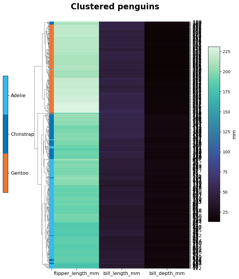
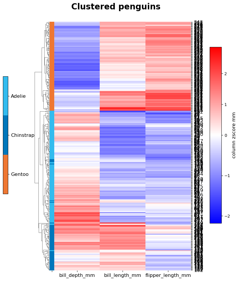
# Let's cluster some penguins based on their measured features, after removing entries with NAs.
non_na_penguins = penguin_df[~penguin_df.isna().values.any(axis=1)]
# Once with the original values and once with z-scoring the columns (flag takes None or the axis).
# The row names will be the index numbers, which are not meaningful here, but suffices for illustration.
for do_z in [None, 0]:
    cmap = 'mako' if do_z is None else 'bwr'
    centre = None if do_z is None else 0
    Heatmaps.clustermap(non_na_penguins, columns=['bill_length_mm', 'bill_depth_mm', 'flipper_length_mm'],
                        row_column='index', z_score=do_z, centre=centre, cbar_label='mm', class_col='species',
                        title="Clustered penguins", plot_out=out_dir+"Penguins_"+str(do_z)+'ZScore', cmap=cmap,
                        x_size=8, y_size=10, row_cluster=True, col_cluster=True, formats=['png'])