Bed Analysis
Analyses related to bed-files, where the peaks are located with respect to genes, how multiple bed-files overlap, or to get a mapping of overlapping peaks between files and genes and more. Centred on the usage of pybedtools, but also works with stored bed-files. To run the example code for this module, we will always start with this block of code:
import Bed_Analysis
from pybedtools import BedTool
out_dir = 'docs/gallery/'  # Replace with wherever you want to store it.
- Bed_Analysis.gene_location_bpwise(bed_dict, gtf_file, plot_path, tss_type='5', external_bed={}, palette='tab20', formats=['pdf'])
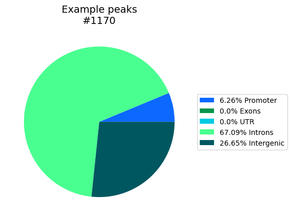
Based on a gtf file builds bed-objects for Promoter (±200bp), Exons, UTRs and Introns, and then counts how many of the bp in the bed file(s) are located within those annotations and which are intergenic. All gene features are exclusive, overlaps are removed. Introns are gene bodies subtracted by all other features. The bed_dict can also be a list of bed files, to omit recreating the gtf-annotations each time. Creates a pie chart with the percentages in the given path. Also returns a dictionary with the bp-location of each bed-region and the total overlaps.
- Parameters:
bed_dict – A dictionary with {title tag: bed-file or BedTools object}
gtf_file – gtf-file in GENCODE’s format, can be gzipped.
tss_type – What to consider as promoter of genes, either ‘5’ to use only the most 5’ TSS, or ‘all’ to consider ±200bp around all annotated TSS of a gene.
external_bed – An additional dictionary of bed-file or BedTools object which will be added as category for the intersection. This will be considered as highest priority, meaning the regions in there are removed from the gene-related features, and a bp overlapping external_bed will not be counted anywhere else. Multiple external bed-regions shouldn’t overlap, that causes undefined outcomes.
- Returns:
regions_locs: For each entry in the bed_dict a dictionary with the bp-wise locations for each individual region.
total_locs: For each entry in the bed_dict the overall overlap of base pairs with each genomic feature.
- Return type:
example_bed_file = "ExampleData/H3K27acPeaks_chr21.narrowPeak"
bed_dict = {'Example peaks': example_bed_file} # Can have multiple entries, producing output for each.
annotation = 'ExampleData/gencode.v38.annotation_chr21Genes.gtf'
# Use a small set of peaks as example.
region_locs, total_locs = Bed_Analysis.gene_location_bpwise(bed_dict=bed_dict, gtf_file=annotation,
plot_path=out_dir, tss_type='5', palette='glasbey_cool', formats=['png'])
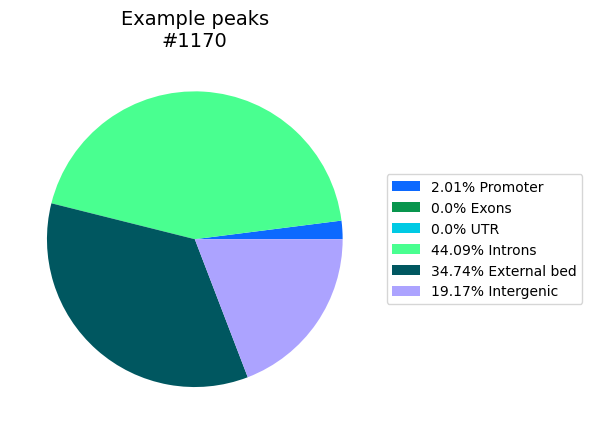
# We can add overlap with an additional bed-file as pie piece. In this example we use a few peaks from the original
# bed-file itself.
external_bed = 'ExampleData/H3K27acPeaks_chr21_subset.narrowPeak.txt'
region_locs, total_locs = Bed_Analysis.gene_location_bpwise(bed_dict=bed_dict, gtf_file=annotation, external_bed={"External bed": external_bed},
plot_path=out_dir+"InclExternal", tss_type='5', palette='glasbey_cool', formats=['png'])
- Bed_Analysis.intersection_heatmap(bed_dict, region_label, plot_path, fisher=False, fisher_background=None, pseudocount=1, annot_nums=True, x_size=16, y_size=10, annot_s=15, col_beds=None, row_beds=None, inter_thresh=1e-09, vmin=None, vmax=None, cmap='plasma', num_cmap='Blues', pickle_path='', tmp_dir='', wspace=0.1, hspace=0.1, n_cores=1, width_ratios=[0.01, 0.05, 0.96], height_ratios=[0.05, 0.97], font_s=16, formats=['pdf'])
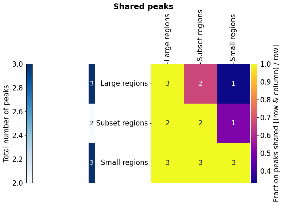
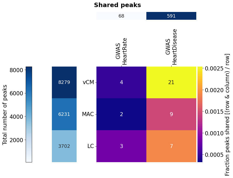
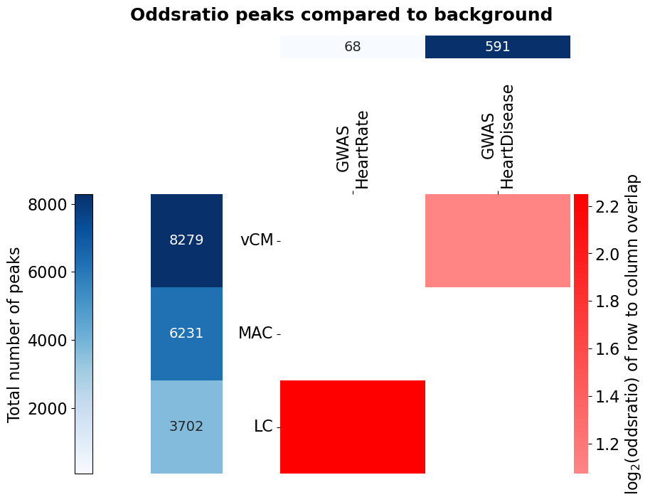
Based on a dictionary {tag: bed_path/BedTools} creates an asymmetric heatmap of the intersection fo each feature, and adds a heatcolumn with the absolute number of regions in the file. Also accepts different bed files/BedTools for rows and columns. The asymmetry of the heatmap overcomes the ambiguity of overlap when the regions are not complete subsets of one another. For example, one region from file A can contain multiple regions from file B, so one value for describing their overlap doesn’t do it justice. The flag fisher allows to additionally run a Fisher’s exact test for the enrichment of the regions versus the columns, but requires a background for each row to compare to. The cells are then coloured by the log2(oddsratio), if the test is significant (p-value ≤ 0.05).
- Parameters:
bed_dict – {tag: bed_path/BedTools}
region_label – label for the regions, e.g. ‘peaks’ or ‘promoter’.
fisher – If True, swap the mode of the function to calculate a two-sided Fisher’s exact test instead of showing the fraction of overlap. Requires to set a background for each of the bed-dict entries used as row: [[row-regions with column overlap, row-regions without column overlap], [background-regions with column overlap, background-regions without column overlap]]
fisher_background – A dictionary of {row_key: BedTool/bed-file} with the background on which the Fisher’s exact test will be calculated for. Any regions in the background overlapping the original row regions is removed before running the test to ensure exclusivity of the groups.
pseudocount – Pseudocount to be added to each cell in the contingency table for the Fisher’s exact test.
annot_nums – If the numbers of intersection should also be written in the cells, else hide.
col_beds – A list of tags from bed_dict that will be shown in the columns. If not given will do all vs all.
row_beds – Same as col_beds but for the rows. Either both or none have to be given.
inter_thresh – Fraction of the region in the row that has to be overlapped by a region in the column to be counted as overlap.
cmap – Colourmap for the intersection heatmap.
num_cmap – Colourmap for the total number of regions.
pickle_path – Path where a pickle object will be stored. If it already exists will be loaded instead to skip the intersection steps. If not given will store it in plot_path.
tmp_dir – Optional path for temporary files created by pybedtools. CARE: If your outer function already uses the same tmp_dir for pybedtools, the objects in there will be deleted.
wspace – Vertical whitespace between plot elements.
hspace – Horizontal whitespace between plot elements.
width_ratios – Control the width ratios of the sub-parts of the plot, meaning the colourbar for the total number of regions, the heatmap of the total number of regions and the heatmap of intersections.
height_ratios – control the height ratios of the plot rows, the first one with the total number of regions of the column beds and the second with the rest.
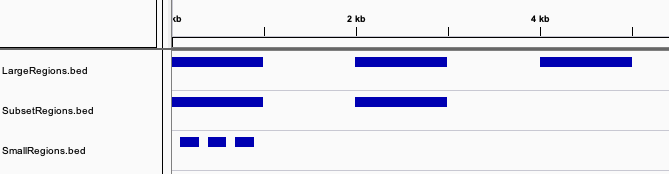
# For the example, let's create three BedTool object that match the image above. The first one with three large regions,
# the second repeating two of those regions, and the last having multiple small regions inside one of those.
large_regions = BedTool('\n'.join(['chr1\t1\t1000', 'chr1\t2000\t3000', 'chr1\t4000\t5000']), from_string=True)
subset_regions = BedTool('\n'.join(['chr1\t1\t1000', 'chr1\t2000\t3000']), from_string=True)
small_regions = BedTool('\n'.join(['chr1\t100\t300', 'chr1\t400\t600', 'chr1\t700\t900']), from_string=True)
multi_bed_dict = {'Large regions': large_regions,
                  'Subset regions': subset_regions,
                  'Small regions': small_regions}
Bed_Analysis.intersection_heatmap(multi_bed_dict, region_label='peaks', plot_path=out_dir, annot_nums=True,  x_size=10, y_size=7,
                           wspace=1.3, hspace=0.7, width_ratios=[0.05, 0.05, 0.96], height_ratios=[0.05, 0.97], formats=['png'])
# Now we repeat the analysis above, but instead of just doing the pairwise-intersection, we make use of the fisher mode
# of the function. For that, we need data with more entries (limited to chr1 though). We use the scATAC-seq data from Hocker 2021 (10.1126/sciadv.abf1444)
# which was aggregated on cell type-level. They defined a union set of ATAC peaks and calculated the RPKM per cell type cluster.
# For four cell types (vCM: ventricular cardiomyocytes, MAC: macrophages, LC: lymphocytes) we subset this union to those peaks with RPKM ≥ 2 in
# the respective cell type. These peaks we then intersect with GWAS SNPs from the GWAS catalog for the traits heart rate
# (EFO_0004326) and immune system disease (EFO_0000540). Since we need a group for comparison for the Fisher's exact test,
# we take all chr1 ATAC peaks as background (the function will remove the foreground peaks from the background).
fisher_bed_dict = {"vCM": 'ExampleData/MultiBedFisher/Hocker2021_ATAC_vCM_chr1.bed',
                   "MAC": 'ExampleData/MultiBedFisher/Hocker2021_ATAC_MAC_chr1.bed',
                   "LC": 'ExampleData/MultiBedFisher/Hocker2021_ATAC_LC_chr1.bed',
                   'GWAS\nHeartRate': 'ExampleData/MultiBedFisher/GWAS_EFO_0004326_heart-rate.txt',
                   'GWAS\nHeartDisease': 'ExampleData/MultiBedFisher/GWAS_EFO_0003777_heart-disease.txt'}
fisher_background = {c: 'ExampleData/MultiBedFisher/Hocker2021_ATAC_Union_chr1.bed' for c in ['vCM', 'MAC', 'LC']}
Bed_Analysis.intersection_heatmap(fisher_bed_dict, region_label='peaks', fisher=True, fisher_background=fisher_background,
                                  row_beds=['vCM', 'MAC', 'LC'], col_beds=['GWAS\nHeartRate', 'GWAS\nHeartDisease'],
                                  plot_path=out_dir+"HockerATAC", annot_nums=True,  x_size=10, y_size=8, n_cores=2,
                                  wspace=0.4, hspace=0.9, width_ratios=[0.05, 0.2, 0.96], height_ratios=[0.08, 0.97], formats=['png'])
Don’t expect a very meaningful result here. The data is limited to chr1 and the activity filter of the peaks per cell type rather crude. Also, please note that if you do overlap with SNVs, you should consider their linkage disequilibrium structure.
- Bed_Analysis.upset_to_reference(bed_files, ref_tag, y_label='Intersecting regions', title_tag='', plot_path='', font_s=16, formats=['pdf'])
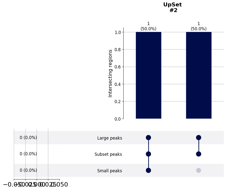
Creates an upsetplot based on the bed_file defined by the ref_tag. That means that the bars will all show the number of reference regions, to avoid ambiguous many-to-one intersections. That also means that the horizontal bars that would normally show the total size of all other comparing bed-files will not be shown (the ugly leftovers one the lower left can be cropped).
- Parameters:
bed_dict – {tag: bed_path/BedTools}
ref_tag – Key in bed_dict to use as the reference.
# Similar to the asymmetric above, this UpSet plot is meant for checking the overlap of bed-files with different sizes.
# However, this one shows the overlap only with respect to one selected bed-file. Let's use the same example bed objects
# as for the previous functions, and show the overlap only with respect to the second set of regions. One of the two
# peaks overlaps with both the large regions and the small regions, and one only with the large regions.
large_regions = BedTool('\n'.join(['chr1\t1\t1000', 'chr1\t2000\t3000', 'chr1\t4000\t5000']), from_string=True)
subset_regions = BedTool('\n'.join(['chr1\t1\t1000', 'chr1\t2000\t3000']), from_string=True)
small_regions = BedTool('\n'.join(['chr1\t100\t300', 'chr1\t400\t600', 'chr1\t700\t900']), from_string=True)
multi_bed_dict = {'Large regions': large_regions,
                  'Subset regions': subset_regions,
                  'Small regions': small_regions}
Bed_Analysis.upset_to_reference(bed_files=multi_bed_dict, ref_tag='Subset regions', y_label='Intersecting regions',
                                plot_path=out_dir, formats=['png'])
- Bed_Analysis.peaks_peaks_overlap(peak_file, other_peak_file)
Intersects two bed-files or BedTools object to return a dictionary with {chr start end: {other peaks}}.
- Parameters:
peak_file – Path to a bed-file or BedTools object of the regions that will be the keys in the mapping dictionary.
other_peak_file – Path or BedTools object to be mapped to peak_file and listed as values in the dictionary.
- Returns:
peak_dict: A dictionary with {chr start end: {other peaks}}. Values are empty if there was no intersection.
- Return type:
# Let's get a mapping of two small example sets of regions where all regions from the second set are located in
# one region of the first set.
large_regions = BedTool('\n'.join(['chr1\t1\t1000', 'chr1\t2000\t3000', 'chr1\t4000\t5000']), from_string=True)
small_regions = BedTool('\n'.join(['chr1\t100\t300', 'chr1\t400\t600', 'chr1\t700\t900']), from_string=True)
peak_peak_map = Bed_Analysis.peaks_peaks_overlap(peak_file=large_regions, other_peak_file=small_regions)
print(peak_peak_map)
{'chr1\t1\t1000': {'chr1\t100\t300', 'chr1\t700\t900', 'chr1\t400\t600'}, 'chr1\t2000\t3000': set(), 'chr1\t4000\t5000': set()}
- Bed_Analysis.peaks_promoter_overlap(peak_file, gtf_file, tss_type='all', gene_set=(), extend=200)
Based on a bed-file path or BedTools object returns a dictionary with {chr start end: {genes whose promoter overlap}} and one with {gene: {peaks}}.
- Parameters:
peak_file – Path to a bed-file or BedTools object of the regions that will be used for the intersection.
gtf_file – gtf-file in GENCODE’s format, can be gzipped.
tss_type – “5” to do the overlap only for the 5’ TSS or “all” to do it for all unique TSS of all transcripts in the gtf-file.
gene_set – Set of Ensembl IDs or gene names or mix of both to limit the output to. If empty, return for all genes in the annotation.
extend – Number of base pairs to extend the TSS in each direction. 200 means a window of size 401.
- Returns:
peak_dict: Dictionary mapping peaks to gene promoters {chr start end: {genes whose promoter overlap}}.
gene_dict: Dictionary doing the mapping the other way around with {gene: {peaks}}.
- Return type:
# Now instead of intersecting multiple bed-files we get the intersection with promoter regions of genes (±200bp around the TSS).
example_bed_file = "ExampleData/H3K27acPeaks_chr21.narrowPeak"
annotation = 'ExampleData/gencode.v38.annotation_chr21Genes.gtf'
peak_promoter_map, promoter_peak_map = Bed_Analysis.peaks_promoter_overlap(peak_file=example_bed_file, gtf_file=annotation, tss_type='5')
print(list(peak_promoter_map.items())[:2])
print(list(promoter_peak_map.items())[:2])
[('chr21\t42974618\t42975047', {'ENSG00000160199'}), ('chr21\t41677496\t41679127', {'ENSG00000227702'})]
[('ENSG00000141956', {'chr21\t41879112\t41879847'}), ('ENSG00000141959', {'chr21\t44299243\t44300860'})]
- Bed_Analysis.peaks_fetch_col(base_regions, pattern, same_peaks=False, fetch_col='log2FC')
Take a bed-file or BedTools object with regions as peaks and intersect it with other peak files defined with a filesystem pattern to get their fetch_col values in the base_regions. Useful for example, if one has multiple differential peak calls and want to map them to a base set of regions. If multiple regions overlap a base region, their average signal is taken. Entries of base peaks without overlap will be filled with NaN.
- Parameters:
base_regions – BedTool’s object or path to a bed file with the regions on which the intersection is centred on.
pattern – File path pattern e.g., DiffPeaks/DiffBind_*.bed, or the path to just one individual file. All files matching that pattern will be used for the intersection. The string at the asterisk will be used as identifier. E.g., DiffPeaks/DiffBind_Macrophages.bed will be identified as Macrophages. The files need to have a header starting with # with fetch_col as column name. If it’s not a path pattern but an individual file, the suffix after the last ‘/’ is used as identifier.
same_peaks – Boolean if the base regions are the same regions as the ones found in the pattern files.
fetch_col – The column name in the files found by pattern to identify from which column the value should be taken.
- Returns:
fill_dict: Nested dictionary of the base_regions as keys and the average of the fetch_col in each of the matched files.
matched_files: List of the identifiers derived from the files matching the pattern.
- Return type:
# Let's assume we have a set of ATAC peaks and found differential ATAC peaks for different conditions.
base_peaks_file = 'ExampleData/BaseATAC_peaks.txt'
# We have a directory with two bed files with a header from which we want to get the average log2FC value in all the
# base peaks they overlap.
diff_atac_pattern = 'ExampleData/DiffATAC/DiffATAC_*.txt'
Take a look at the example ATAC peaks and the files defined by the file system pattern. BaseATAC_peaks.txt
chr1    1       1000
chr1    2000    3000
chr1    4000    5000
DiffATAC/DiffATAC_Macs.txt
#chr    start   end     log2FC
chr1    20      50      -2
chr1    400     500     -4
chr1    2010    2050    2
DiffATAC/DiffATAC_TCells.txt
#chr    start   end     log2FC
chr1    4000    4500    3
chr1    900     1100    5
base_peaks_log2fc, matched_ids = Bed_Analysis.peaks_fetch_col(base_regions=base_peaks_file, pattern=diff_atac_pattern, same_peaks=False, fetch_col='log2FC')
print(base_peaks_log2fc)
{'chr1\t1\t1000': {'Macs': -3.0, 'TCells': nan}, 'chr1\t2000\t3000': {'Macs': 2.0, 'TCells': nan}, 'chr1\t4000\t5000': {'Macs': nan, 'TCells': 3.0}}
- Bed_Analysis.promoter_fetch_col(pattern, gtf_file, tss_type='all', extend=200, gene_set=(), fetch_col='log2FC')
Gets the promoter regions of genes and intersects them with peak files defined with a filesystem pattern to get their fetch_col values in the promoters. Useful for example, if one has multiple differential peak calls and wants to know the log2FC in promoters. If multiple regions overlap a promoter, their average signal is taken. Entries of promoters without overlap will be filled with NaN.
- Parameters:
pattern – File path pattern e.g., DiffPeaks/DiffBind_*.bed, or the path to just one individual file. All files matching that pattern will be used for the intersection. The string at the asterisk will be used as identifier. E.g., DiffPeaks/DiffBind_Macrophages.bed will be identified as Macrophages. The files need to have a header starting with # with fetch_col as column name. If it’s not a path pattern but an individual file, the suffix after the last ‘/’ is used as identifier.
gtf_file – gtf-file in GENCODE’s format, can be gzipped.
tss_type – “5” to get only the 5’ TSS or “all” to get all unique TSS of all transcripts in the gtf-file. When ‘all’, values are averaged across multiple promoters.
extend – Number of base pairs to extend the TSS in each direction. 200 means a window of size 401.
gene_set – Set of Ensembl IDs or gene names or mix of both to limit the output to. If empty, return for all genes in the annotation.
fetch_col – The column name in the files found by pattern to identify from which column the value should be taken.
- Returns:
gene_values: Nested dictionary of the Ensembl IDs as keys and the average of the fetch_col in each of the matched files.
matched_files: List of the identifiers derived from the files matching the pattern.
- Return type:
# This one is very similar to the previous, but starts from genes to get their promoter regions to then get the
# values from other bed files in those promoters.
diff_atac_pattern = 'ExampleData/DiffATAC/DiffATAC_*.txt'
annotation = 'ExampleData/gencode.v38.annotation_chr21Genes.gtf'
promoter_log2FC, matched_ids = Bed_Analysis.promoter_fetch_col(pattern=diff_atac_pattern, gtf_file=annotation, tss_type='5',
                                                               gene_set={'ENSG0000MOCK1', 'ENSG0000MOCK2'}, fetch_col='log2FC')
print(promoter_log2FC)
{'ENSG0000MOCK2': {'Macs': nan, 'TCells': 5.0}, 'ENSG0000MOCK1': {'Macs': -4.0, 'TCells': nan}}
- Bed_Analysis.peaks_genebody_overlap(peak_file, gtf_file, gene_set=())
Based on a bed-file path or BedTools object returns a dictionary with {gene: fraction of gene body overlapping with peak_file}.
- Parameters:
peak_file – BedTool’s object or path to a bed file with the regions on which the intersection is centred on.
gtf_file – gtf-file in GENCODE’s format, can be gzipped.
gene_set – Set of Ensembl IDs or gene names or mix of both to limit the output to. If empty, return for all genes in the annotation.
# Based on an example peak file and gtf-file, we get the fraction of the gene body that is covered by the peaks.
peak_file = 'ExampleData/H3K27acPeaks_chr21.narrowPeak'
annotation = 'ExampleData/gencode.v38.annotation_chr21Genes.gtf'
gene_body_fractions = Bed_Analysis.peaks_genebody_overlap(peak_file=peak_file, gtf_file=annotation,
                                                          gene_set=['ENSG00000275895', 'ENSG00000273840'])
print(gene_body_fractions)
{'ENSG00000275895': 0.017215466593796965, 'ENSG00000273840': 0.001927173966075233}
- Bed_Analysis.possible_interactions(peak_file, gtf_file, extend=2500000, gene_set={}, tss_type='all')
Take a bed-file or BedTools object along with a gtf-file annotation to find all possible interactions, meaning all pairs of CRE-gene that are within the extend limit.
- Parameters:
peak_file – Path to a bed-file or a BedTools object.
gtf_file – gtf-file in GENCODE’s format, can be gzipped.
extend – Number of base pairs to extend the TSS in each direction. 200 means a window of size 401.
gene_set – Set of Ensembl IDs or gene names or mix of both to limit the output to. If empty, return for all genes in the annotation.
tss_type – “5” to get only the 5’ TSS or “all” to get all unique TSS of all transcripts in the gtf-file.
- Returns:
all_interactions: All CRE-gene pairs within the defined distance, separated by a hash sign, e.g. chrX-100636854-100637354#ENSG00000000003.
- Return type:
# For a small example, get all possible region-gene combinations within 500 base pairs.
peak_file = 'ExampleData/H3K27acPeaks_chr21.narrowPeak'
annotation = 'ExampleData/gencode.v38.annotation_chr21Genes.gtf'
all_interactions = Bed_Analysis.possible_interactions(peak_file=peak_file, gtf_file=annotation, extend=500, tss_type='5')
print(list(all_interactions)[:3])
['chr21-37073278-37074479#ENSG00000185808', 'chr21-28993136-28993479#ENSG00000198862', 'chr21-45404209-45405005#ENSG00000273796']